통계학에서의 중심경향이란 확률분포에서의 중심을 의미하는데 평균, 중심, 중간, 최대빈도 값 등등 어떤 것으로 규정할지 헷갈린다.

가장 익숙한 것이 Mean(평균), Median(가운데), Mode(최빈값)이다.
유추할 수 있겠지만, 아래 예시로 다시 한번 확인해보자.
Counter는 어디가 가운데인지 측정하기 위한 '자'라고 생각하면 된다.
각각을 계산해보면,
Mean: (1+1+2+3+4+5+6+6+6+10+10) / 11 = 4.9
Median: date_6 = 5
Mode: 6
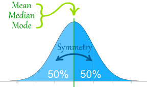
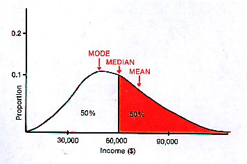
참고로 정규분포(normal distribution)의 경우에는 아래와 같은 모양일 것이다.

가장 익숙한 것이 Mean(평균), Median(가운데), Mode(최빈값)이다.
유추할 수 있겠지만, 아래 예시로 다시 한번 확인해보자.
data: 1-1-2-3-4-5-6-6-6-10-10
counter: 1-2-3-4-5-6-7-8-9-10-11
Counter는 어디가 가운데인지 측정하기 위한 '자'라고 생각하면 된다.
각각을 계산해보면,
Mean: (1+1+2+3+4+5+6+6+6+10+10) / 11 = 4.9
Median: date_6 = 5
Mode: 6
참고로 정규분포(normal distribution)의 경우에는 아래와 같은 모양일 것이다.
- Arithmetic mean or simply, mean
- the sum of all measurements divided by the number of observations in the data set.
- Median
- the middle value that separates the higher half from the lower half of the data set. The median and the mode are the only measures of central tendency that can be used for ordinal data, in which values are ranked relative to each other but are not measured absolutely.
- Mode
- the most frequent value in the data set. This is the only central tendency measure that can be used with nominal data, which have purely qualitative category assignments.
- Geometric mean
- the nth root of the product of the data values, where there are n of these. This measure is valid only for data that are measured absolutely on a strictly positive scale.
- Harmonic mean
- the reciprocal of the arithmetic mean of the reciprocals of the data values. This measure too is valid only for data that are measured absolutely on a strictly positive scale.
- Weighted arithmetic mean
- an arithmetic mean that incorporates weighting to certain data elements.
- Truncated mean or trimmed mean
- the arithmetic mean of data values after a certain number or proportion of the highest and lowest data values have been discarded.
- Interquartile mean
- a truncated mean based on data within the interquartile range.
- Midrange
- the arithmetic mean of the maximum and minimum values of a data set.
- Midhinge
- the arithmetic mean of the two quartiles.
- Trimean
- the weighted arithmetic mean of the median and two quartiles.
- Winsorized mean
- an arithmetic mean in which extreme values are replaced by values closer to the median.
Any of the above may be applied to each dimension of multi-dimensional data, but the results may not be invariant to rotations of the multi-dimensional space. In addition, there are the
- Geometric median
- which minimizes the sum of distances to the data points. This is the same as the median when applied to one-dimensional data, but it is not the same as taking the median of each dimension independently. It is not invariant to different rescaling of the different dimensions.
- Quadratic mean (often known as the root mean square)
- useful in engineering, but not often used in statistics. This is because it is not a good indicator of the center of the distribution when the distribution includes negative values.
- Simplicial depth
- the probability that a randomly chosen simplex with vertices from the given distribution will contain the given center
- Tukey median
- a point with the property that every halfspace containing it also contains many sample points
- https://en.wikipedia.org/wiki/Central_tendency
댓글
댓글 쓰기